In the realm of mathematical finance there are two relatively disjoint worlds: the “buy-side” and the “sell-side”. Buyers are analyzing the available financial products (e.g. stocks, bonds, derivatives, etc.) and are trying to predict, and profit off of, the future prices of these assets—i.e. they are trying to estimate the real-world probability distribution, commonly denoted $P$, of the future stochastic price movements.
On the other side, sellers (aka market-makers) are trying to set a fair price for more illiquid assets, like derivatives, using the prices of more liquid assets, like stocks, which are priced by supply and demand. One particular challenge is that investors all have different risk preferences. One way to quantify this risk is with the sharp ratio, which measures risk relative to a numeraire, like a US treasury security, which has a risk-free rate of return $r$. One model for the price of derivative is to use a stochastic discount factor (SDF), also called a pricing kernel, $M_t$. The price $F$ of a derivative at time $t$, which pays out at future time $T$, is then given by
$$ F_t = \mathbf{E}_{P}\left[M_T F_T\right] = e^{-r(T-t)} \mathbf{E}_{Q}\left[ F_T \right] $$
Where in the last step we factored out the risk-free interest and merged the SDF into the probability measure. This is allowed given the measures are equivalent—written $P \sim Q$—and we assume no arbitrage exists; the fundamental theorem of asset pricing encapsulates this.
Pricing derivatives using the risk-neutral measure $Q$ comes with a few advantages over the real world measure $P$. For one, it is often simpler—requires fewer parameters, and we don’t need to worry about SDF—to calibrate pricing models; two, as we will see, the underlying asset becomes a martingale w.r.t. $Q$; lastly, we don’t need to account for investors specific risk preferences.
preliminaries
Let’s get some definitions out of the way before deriving the main result below. We will start with the definition of a martingale process, and then define what is required for two probability measures to be called equivalent.
For the remainder of the article we will work on the probabilty space $(\Omega, \mathcal{F}, \{\mathcal{F_t}\}, P)$, where $\Omega$ is the sample space of possible paths, $\mathcal{F}_t$ is the filtration (think available information) of the $\sigma$-algebra $\mathcal{F}$ up to time $t$, and $P$ is the probability measure on the sample space.
Note that a sample path, denoted $\omega \in \Omega$, allows us to think of stochastic variables, given a sample path, as deterministic functions of time: $t \mapsto X_t(\omega)$
martingales
Intuitively a martingale process is one which is not biased, i.e. it does not drift. This can be made rigorous by requiring that on a stochastic process $Y_t$ satisfies (using a generalization of conditional expectation)
$$ \mathbf{E}_P[Y_t | \mathcal{F}_s] = Y_s $$
for $s < t$. This says that the conditional expectation of the future value, given the present information, will always be equal to the present value.
For Ito processes, it is sufficient that the drift term is zero.
equivalence of measures
A probability measure is not unique on a sample space is not unique; changing measures requires some notion of equivalence. Chiefly, if we want to transform $P \to Q$, we must have
$$ P(H) = 0 \implies Q(H) = 0 $$
for all $H \in \mathcal{F}_T$, where we fix $t = T$. We then say $Q$ is absolutely continuous w.r.t. $P$ and write $Q \ll P$, which by the Radon-Nikodym theorem occurs only if
$$ dQ(\omega) = Z_T(\omega)dP(\omega) $$
Here our $Z_T(\omega) = Z_t(\omega) > 0$ a.s., which implies $P\ll Q$, allowing us to assert equivalence and write $P \sim Q$.
Girsanov’s theorem
Given an Ito process $X_t$ on the probability space $(\Omega, \mathcal{F}, \{\mathcal{F}_t \}, P)$, described by the stochastic differential equation
$$ dX_t = \mu(t, \omega) dt + \sigma(t,\omega)dW_t \tag{1} $$
where $\omega \in \Omega$ represents a sample path in the sample space of all possible paths, $\mathcal{F}_t$ is the filtration of the $\sigma$-algebra $\mathcal{F}$ up to time $t$ (not actually important for what are we are doing), and most importantly $W_t$ is a wiener process (brownian motion) with respect to the measure $P$.
Let’s now define a new process
$$ Z_t = \exp \left( -\int_0^t u(s, \omega) dW_s - {1 \over 2} \int_0^t u(s, \omega)^2 ds \right), $$
which satisfies the following SDE, where we now make the simplifying assumption that $u(t, \omega) = u(t)$—i.e. it is deterministic—
$$ dZ_t = -u(t) Z_t dW_t. $$
Now, if we use the product rule for Ito calculus
$$ d(X_t Y_t) = Y_t dX_t + X_t dY_t + dX_t dY_t $$
and if we assume $\mu(t)$ and $\sigma(t)$, found in (1), are deterministic, and define u(t) by
$$ \mu(t) - \sigma(t) u(t) = \alpha(t); $$
In general, for an $n$-dimensional Ito process, in terms of an $m$-dimensional Wiener process $W_t$, $\mu \in \mathbb{R}^n$, $\sigma \in \mathbb{R}^{n\times m}$, and $u \in \mathbb{R}^m$. So in higher dimensions invertability of $\sigma$ becomes an issue, but that will not be discussed here.
so, with X_t defined in (1), we find that the process $Y_t = Z_t X_t$, where, importantly (for simulation purposes), the noise process $W_t$ is shared, satisfies
$$ dY_t = d(Z_t X_t) = \alpha(t) Z_t dt + (Z_t \sigma(t) - Y_t u(t)) dW_t $$
Which means, WLOG, we can make $Y_t$ a martingale by choosing $\alpha(t) = 0$, eliminating the drift term. In $n = m = 1$ dimensions, we then have $u(t) = {\mu(t) \over \sigma(t)}$.
the risk-neutral measure
Looking at the above derivation, as well as the definition for equivalence of measures we can define an equivalent martingale measure, or risk-neutral measure, $Q$ on a derivative paying out at time $T$ modeled by an Ito process, by
$$ dQ = \exp \left( -\int_0^T u(s,\omega)dW_s - {1 \over 2}\int_0^T u^2(s,\omega)ds \right)dP, $$
since, accounting for the discount rate,
$$ \begin{align*} \mathbf{E}_P\left[ Z_T e^{-rT}X_T\right] &= e^{-rT}\mathbf{E}_P\left[ Z_T X_T\right] \\\ &= e^{-rT}\mathbf{E}_Q\left[ X_T\right] \end{align*} $$
We can also check that $Q$ is indeed a probability measure:
$$ \mathbf{E}_Q[1] = \mathbf{E}_P[Z_t] = \mathbf{E}_P[Z_0] = \mathbf{E}_P[1] = 1 $$
using the fact that $Z_t$ is a martingale.
final thoughts and a visualization
This machinery gives us a way to calculate risk neutral expectations: calibrate $Z_t$ by fitting the parameters of a model for the underlying asset and use that measure to calculate expectations of more complicated derivatives. In practice there are fancier tricks, that I may eventually deliberate on.
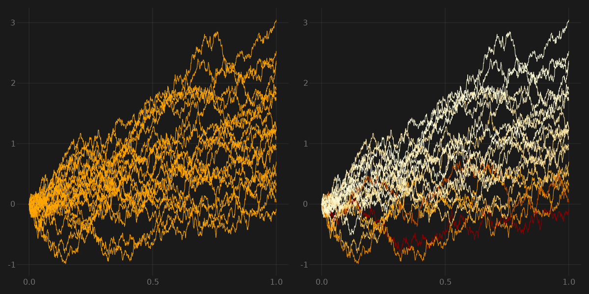
Intuitively, the risk-neutral measure doesn’t change the paths of the process, it just weights the paths s.t. the expectation over all paths is equal to the starting position. For a simple model this looks like this:

This plot was generated with a $1$-dimensional Ito process with $\mu = 1.5$ and $\sigma = 1$. Code can be found here.