The transmon qubit, first proposed in 2007 by Koch et al. 1, has become a top contender for realizing large-scale NISQ devices. The transmon is based on an anharmonic oscillator realized by a Josephson junction shunted to a capacitor. Anharmonicity — i.e. unevenly separated energy levels, c.f. the harmonic oscillator — is the key ingredient enabling a stable two-level subsystem where the qubit state will live.
The circuit diagram (taken from 1), shown below,

consists of a Josephson junction element shunted by a capacitor. For a detailed description of this system and quantum electrical circuits in general, see 2.
lab-frame Hamiltonian
Without going into all the details of this circuit (see 1 for more), the simplified Hamiltonian for this system is given by
$$ \begin{equation} \hat{H} = 4E_C \hat{n}^2 - E_J \cos (\hat{\varphi}) \end{equation} $$
where $\hat{n}$ is the charge number operator and $\hat{\varphi}$ is the phase operator; $\hat{n} \equiv \partial_{\hat{\varphi}}$ and $\hat{\varphi}$ are canonically conjugate variables. The first term is the charging energy of the capacitor and the second term is the Josephson energy. We refer to this as the cosine Hamiltonian.
For small $\varphi$, i.e. weak anharmonicity, we can approximate (1) by expanding the cosine term to fourth order:
$$ \begin{equation} \hat{H} = 4E_C \hat{n}^2 - E_J \left( 1 - {\hat{\varphi}^2 \over 2} + {\hat{\varphi}^4 \over 24} \right) \end{equation} $$
Using $\hat{n} = {i \over 2} \sqrt[4]{E_J \over 2E_C}(\hat{a}^\dag - \hat{a})$ and $\hat{\varphi} = \sqrt[4]{2E_C \over E_J}(\hat{a}^\dag + \hat{a})$, we can rewrite the Hamiltonian (dropping constant terms, see 2 for details) with the annihilation and creation operators $\hat{a}$ and $\hat{a}^\dag$:
$$ \begin{equation} \hat{H} = \omega_0 \hat{a}^\dag \hat{a} - {\delta \over 12} \left(\hat{a} + \hat{a}^\dag \right)^4 \end{equation} $$
where $\omega_0 = \sqrt{8E_J E_C}$ is the unshifted resonant frequency of the oscillator and $\delta = E_C$ is the anharmonicity. We refer to this as the quartic Hamiltonian.
Note: the transmon being only weekly anharmonic means leakage errors will be significant when driving the qubit with large amplitudes.
At this point in the derivation of the typical transmon Hamiltonian, a lot of handwaving is used to disappear a number of terms in (3), using the rotating wave approximation (RWA) as justification. The resulting Hamiltonian is
$$ \begin{equation} \boxed{ \hat{H}_{\text{transmon}} = \omega \hat{a}^\dag \hat{a} - {\delta \over 2} \hat{a}^\dag \hat{a}^\dag \hat{a} \hat{a} } \end{equation} $$ where $\omega = \omega_0 - \delta$ is the shifted resonant frequency of the oscillator.
We can also add an on resonance driving term to the transmon Hamiltonian of the form
$$ \begin{equation} \hat{H}_d(t) = \Omega(t)\left(e^{i (\omega t + \phi(t))} \hat{a} + e^{-i (\omega t + \phi(t))} \hat{a}^\dag \right) \end{equation} $$
where $\Omega(t)$ is the amplitude of the drive and $\phi(t)$ is the phase. This Hamiltonian is referred to as the duffing oscillator Hamiltonian.
rotating wave approximation
To understand the rotating wave approximation (RWA) it is necessary to understand unitary transformations in quantum mechanics. Let’s say we want to transform a state unitarily, i.e,
$$ \psi(t) \to \psi’(t) = U(t) \psi(t) $$
then, using the Schrodinger equation, we find that the Hamiltonian must transform as
$$ \hat{H} \to \hat{H}’ = U\hat{H} U^\dag + i \dot{U} U^\dag $$
which is a type of gauge transformation (see my post on ghosts, gauges, and generating functionals for an example in QFT).
Now, using communtation properties of the ladder operators $\hat{a}$ and $\hat{a}^\dag$, namely $[\hat{a}, \hat{a}^\dag] = 1$, we can write the transmon Hamiltonian in (4) as
$$ \begin{equation} \hat{H} = \omega \hat{n} + {\delta \over 2} \hat{n} (\hat{n} - 1) \end{equation} $$
where $\hat{n} = \hat{a}^\dag \hat{a}$ is the number operator. Using the unitary transformation $U(t) = e^{i \omega t \hat{n}}$ — moving into the rotating frame of the transmon at the resonant frequency — we can transform the Hamiltonian to
$$ \begin{aligned} \hat{H} \to \hat{H}’ &= U(t) \hat{H} U^\dag(t) + i \dot{U} U^\dag \\ &= e^{i \omega t \hat{n}} \left( \omega \hat{n} + {\delta \over 2} \hat{n} (\hat{n} - 1) \right) e^{-i \omega t \hat{n}} - \omega \hat{n} \\ &= {\delta \over 2} \hat{n} (\hat{n} - 1)\\ \end{aligned} $$
since $[e^{i \omega t \hat{n}}, \hat{n}] = 0$.
The drive term in (5) transforms as:
$$ \begin{aligned} \hat{H}_d(t) \to \hat{H}’_d(t) &= U(t) \hat{H}_d(t) U^\dag(t) \\ &= \Omega(t) \left( e^{i (\omega t + \phi(t))} U(t) \hat{a} U^\dag(t) + e^{-i (\omega t + \phi(t))} U(t) \hat{a}^\dag U^\dag(t) \right) \\ &= \Omega(t) \left( e^{i \phi(t)} \hat{a} + e^{-i \phi(t)} \hat{a}^\dag \right) \\ \end{aligned} $$
where we have used $e^{i \omega t \hat{n}} \hat{a} e^{-i \omega t \hat{n}} = e^{-i\omega t}\hat{a} $ and $e^{i \omega t \hat{n}} \hat{a}^\dag e^{i \omega t \hat{n}} = e^{i\omega t} \hat{a}^\dag $.
Note: The identity $e^{i \omega t \hat{n}} \hat{a} e^{-i \omega t \hat{n}} = \hat{a} e^{-i\omega t}$ can be derived using the Baker-Campbell-Hausdorff formula:
$$ \begin{aligned} e^X Y e^{-X} &= Y + [X, Y] + {1 \over 2!} [X, [X, Y]] + {1 \over 3!} [X, [X, [X, Y]]] + \cdots \\ &= \sum_{n=0}^\infty {1 \over n!} \underbrace{[X, [X, \cdots [X}_{n \text{ times}}, Y]] \cdots ] \\ &= \sum_{n=0}^\infty {1 \over n!} (\operatorname{ad}_X)^n (Y) \\ \end{aligned} $$
where $\operatorname{ad}_X$ is the adjoint operator defined as $\operatorname{ad}_X(Y) = [X, Y]$. In our case, $X = i \omega t \hat{n}$ and $Y = \hat{a}$, so
$$ \begin{aligned} (\operatorname{ad}_{i \omega t \hat{n}})^n (\hat{a}) &= [i \omega t \hat{n}, [i \omega t \hat{n}, \cdots [i \omega t \hat{n}, \hat{a}]] \cdots ] \\ &= (i \omega t)^n (\operatorname{ad}_{\hat{n}})^n (\hat{a}) \\ &= (i \omega t)^n (-1)^n \hat{a} \\ &= (-i \omega t)^n \hat{a} \\ \end{aligned} $$
using $[\hat{n}, \hat{a}] = -\hat{a}$, yielding
$$ \begin{aligned} e^{i \omega t \hat{n}} \hat{a} e^{-i \omega t \hat{n}} &= \sum_{n=0}^\infty {1 \over n!} (-i \omega t)^n \hat{a} \\ &= e^{-i \omega t} \hat{a}. \\ \end{aligned} $$
Similarly, since $[\hat{n}, \hat{a}^\dag] = \hat{a}^\dag$, $e^{i \omega t \hat{n}} \hat{a}^\dag e^{-i \omega t \hat{n}} = e^{i \omega t} \hat{a}^\dag$.
With this we can see why terms such as $\hat{a} \hat{a} \hat{a} \hat{a}$ and $\hat{a}^\dag \hat{a} \hat{a} \hat{a}$ disappear going from equation (3) to equation (4), using the RWA; the unitary transformation leaves fast oscillating factors attached to those terms.
rotating-frame Hamiltonian
Putting together all of the pieces above we arrive at the following Hamiltonian for the transmon in the rotating frame:
$$ \begin{equation} \boxed{ \hat{H}^{\text{RWA}}_{\text{transmon}}(t) = {\delta \over 2} \hat{a}^\dag \hat{a}^\dag \hat{a} \hat{a} + u(t)\hat{a} + u^*(t) \hat{a}^\dag } \end{equation} $$
where $u(t)$ is a complex-valued control function that can be used to drive the transmon.
Note: To accomadate numerical optimization methods that require real-valued control functions, we can rewrite the drive term $\hat{H}_d^{\text{RWA}}$ in (8) as $$ \begin{equation} \hat{H}^{\text{RWA}}_d(t) = u_1(t) (\hat{a} + \hat{a}^\dag) + u_2(t) i (\hat{a} - \hat{a}^\dag) \end{equation} $$ where we used $u(t) = u_1(t) + i u_2(t)$.
qubit subspace
Staring at equation (7), it becomes apparent that if we restrict ourselves to two levels (which is where we typically want our state populations to live when building qubits), $\hat{a}^\dag \hat{a}^\dag \hat{a} \hat{a} = 0$, $\hat{a} + \hat{a}^\dag = X$, and $i(\hat{a} - \hat{a}^\dag) = -Y$, and we find ourselves with the following Hamiltonian:
$$ \begin{equation} \hat{H}(t) = u_1(t) X + u_2(t) Y \end{equation} $$
where $X$ and $Y$ are the Pauli matrices. And, since $[X, Y] \propto Z$, this Hamiltonian is fully controllable — this is a technical point, which in the quantum setting says that the Lie subalgebra generated from the control Hamiltonians is equal to the full Lie algebra for $SU(2)$, and I will hopefully elucidate this in a later post — which means that realizing any single qubit gate is trivial.
frame errors
Anyway, this is all idealized thinking, as the transmon is not a two-level system, we are using an approximation in a rotating frame, and we began by truncating a cosine term in the original Hamiltonian (1) to fourth order. We have various errors to account for; let’s look at one of them: error arising from the rotating frame approximation, both in the lab frame and in the rotating frame.
Note: in the following we utilize the following unitary fidelity function: $$ \begin{equation} \mathcal{F}(U, U_{\text{goal}}) = \left| \text{tr}\left( U^\dag U_{\text{goal}} \right) \right|^2 \end{equation} $$ where $U$ is in the computational subspace, extracted from the full system unitary.
rotating frame
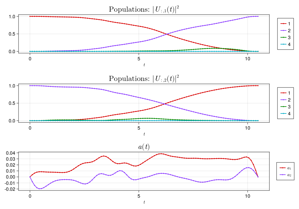
We begin by optimizing a pulse using Piccolo.jl to drive a transmon and realize and $X$ gate in the qubit subspace of a 4-level transmon in the rotating frame, i.e., using equation (7). We get the following pulse with $\mathcal{F} = 0.99996$:
lab frame: duffing
Rolling out in the lab frame of a 9-level transmon — using a carrier wave at the qubit transmon frequency and upsampling the pulse to account for nyquist sampling errors — with the duffing Hamiltonian in equation (4), we get the following pulse with $\mathcal{F} = 0.90135$:
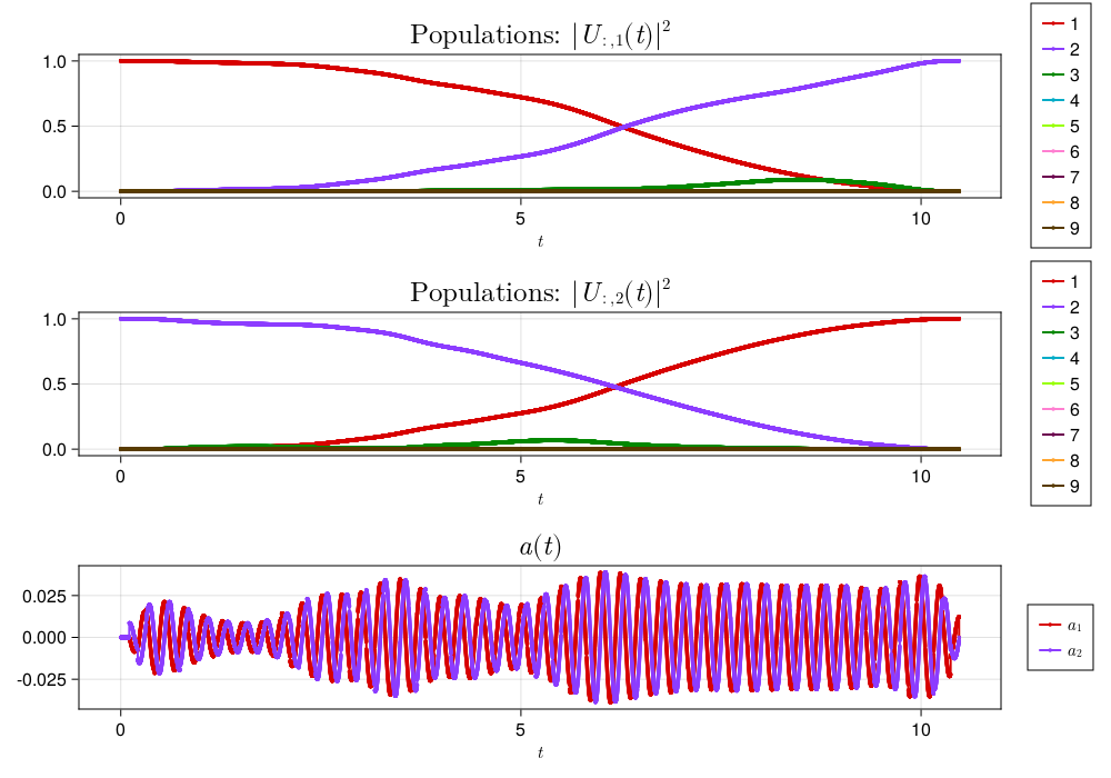
A noticeable, but anticipated (at least ignoring the magnitude), drop in fidelity.
lab frame: quartic
Using the quartic Hamiltonian in equation (3), we get the following pulse with $\mathcal{F} = 0.75057$:
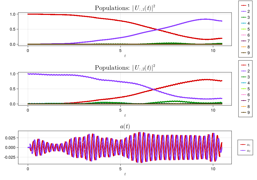
A further, and significant, drop in fidelity, also possibly expected.
lab frame: cosine
Finally, using the cosine Hamiltonian in equation (1), we get the following pulse with $\mathcal{F} = 0.87198$:
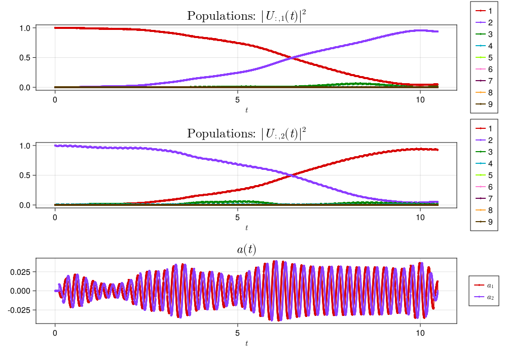
Interestingly, the fidelity is higher than the quartic Hamiltonian but lower than the duffing Hamiltonian.
conclusions
We have derived the typical transmon Hamiltonian, the duffing oscillator, and used the result to optimize an $X$ gate pulse in the rotating frame. Upon rolling this pulse out in the lab frame we see some interesting results:
| Hamiltonian | $\mathcal{F}(U_T, X)$ |
|---|---|
| rotating (eq. 7) | 0.99996 |
| duffing (eq. 4) | 0.90135 |
| quartic (eq. 3) | 0.75057 |
| cosine (eq. 1) | 0.87198 |
It appears that ignored Hamiltonian elements play a significant role, and given that the simulation cost for all of these models was essentially equal, it begs the question, why not use the full Hamiltonian?
Koch, Jens, et al. “Charge-insensitive qubit design derived from the Cooper pair box.” arXiv:cond-mat/0703002 (2007). ↩︎ ↩︎ ↩︎
Ciani, Alessandro, et al. “Lecture Notes on Quantum Electrical Circuits.” arXiv:2312.05329 (2019). ↩︎ ↩︎